Polarization Efficiency Analysis: July 2006 run
I have used data from files sharc2-0326[45-85].fits to estimate the
SHARP polarization efficiency and zero angle of the HWP. Bottom line:
I am not impressed with the precision of the efficiency measurement which ranges from 76% to 120% depending on the data-set.
However, the zero angle measurement is quite good and consistent with
Giles "Quick-check"
procedure.
I have made no attempt to correct for response differences obvious
from the different signals measured when the HWP was at the same
position. Nor have I attempted to look and correct for the effects of
nonlinear bolometer response.
For each file the signal is corrected using the RGM we generated in
January (which was not significantly different from that measured in
July). Next a sum (H+V) and difference (H-V) signal for each
time sample (28 Hz) is generated for all good SHARP pixels. Samples which
sharcsolve labels as bad were removed and missing/widow pixels were
tracked throughout the process. A polarization signal (H-V)/(H+V) and
uncertainty were calculated using the mean and standard deviation of
the sampled difference and sum signals.
The plots below show this polarization signal as a function of the
HWP encoder reading. The signal and error bar are a weighted mean of
the 3 pixels in the center of the the SHARP array. Note that the peak
signals in the H and V halves of the SHARC-II array were not aligned
but were located about half-way between pixles (26,6) and (26,7) for
the V-array and pixel (7,6) for the H-array [pixel coordinate system
starts with (1,1) and ends with (12,32)]. The 3 SHARP pixels used for
the average were (6,6), (7,6), and (6,7) [pixel (7,7) is a widow].
Increasing the number of pixels to a 3 × 3 region cuts the
measured polarization amplitude by about a factor of 1.5 - 2.
Fit curves are of the form S = P cos[4(θ-δ)] = q
cos(4θ) + u sin(4θ) where q = P cos(4δ), u = P
sin(4δ), θ is the HWP encoder reading, and δ is the
offset. The fits are reported in the plots as P = sqrt(q2 +
u2), δ = HWP zero angle = 0.25 * atan(u/q). Uniform
weights are used in all fits; reported χ2 are total,
not per degree of freedom.
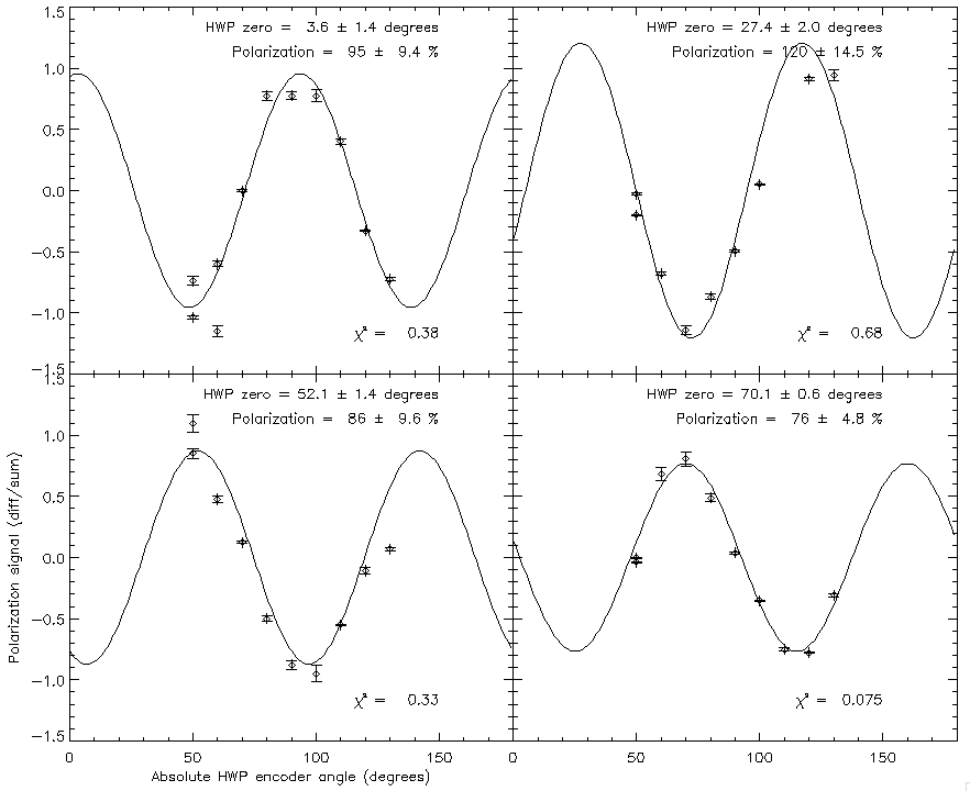
Top Left: Wire grid vertical (0). Top right: wire grid diagonal
between (45). Bottom left: Wire grid horizontal (90). Bottom right:
wire grid diagonal (135). After correcting for the angle of the grid
the mean offset angle w.r.t. vertical is 4.6°. The plot below
does a simultaneous fit for all 4 different grid angles.
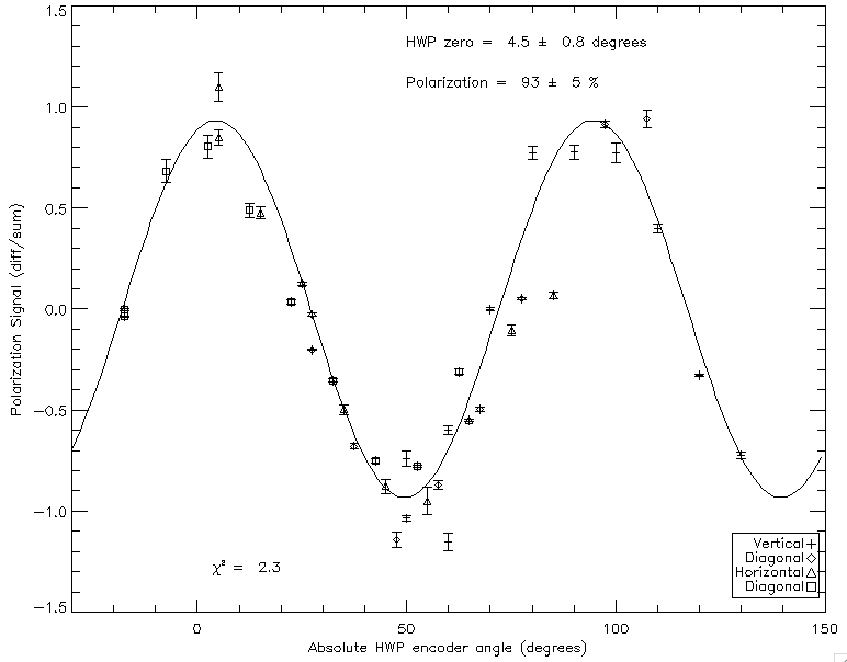
The plot above corrects the HWP encoder angle for the angle of the
wire grid and plots all data w.r.t. the vertical direction. The
results of the combined fit are P = 93 ± 5 % at an offset angle
of δ = 4.5° ± 0.8°.
Using Giles notation from an earlier memo these results give
V_null_encoder = 4.5° = 94.5°
V_null_rel = 4.5° - 50° = -45.5°
HWP zero angle = 2 × -45.5° = -91° = 89°
The previous "Quick-check" procedure gave a value of V_null_encoder = 92.5°
and HWP_zero_angle = 85°
Last updated by John Vaillancourt. 2006-Nov-7.
Return to SHARP analysis logbook.
Return to SHARP home page.