SPARO, the Submillimeter Polarimeter for Antartic Remote Observations, obtained its first polarimetry data, as well as a large amount of photometry data, during the austral winter 2000. The ultimate goal of SPARO is to map the magnetic field of the galactic center on a large scale; however, a smaller goal is the calibration of its photometric observations. First, it was necessary to measure a correction to the atmospheric absorption constant, tau. From there a general constant Y could be measured to calibrate in Jy. Once these constants were determined, SPARO would be capable of making physical measurements of flux.
As there were no observable planet candidates in the austral winter sky, several observations were made of Ngc 6334 and Rcw 57. An estimated flux of Ngc 6334 was obtained from The Astrophysical Journal, in a paper written by Daniel Y. Gezari. His 400 micron observations were made at Mauna Kea, Hawaii with a 5' chopper throw and a 48'' beam. This had to be corrected for SPARO, which observes at 450 microns with a 5 degree chopper throw and has an estimated 5' beam. A source flux for Ngc 6334 could then be estimated at 12,423.25 Jy (+/- 1446.35 Jy).
The signal, S, should depend on tau, the source flux, So, and z, the zenith angle, according to the following equation:
Y is the calibration constant and X is the constant to correct for the Tipper at AST/RO's tau measurement. The Tipper at AST/RO gives a direct measure of tau for a passband centered at 350 microns, but SPARO's passband is centered at 450 microns. Thus, since the atmosphere has a similar but slightly different transmission at these two wavelengths, a correctional factor X must be measured. The signal is measured in integ-units, which is an arbitrary unit the data system assigns it. Plotting the ln S vs. -tau * sec z, X should emerge as the slope, and Y should be obtained from the y-intercept (ln So Y).
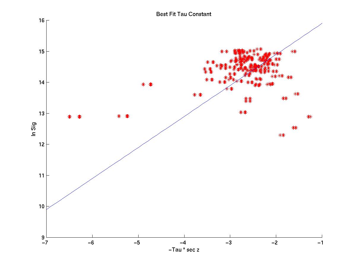
Since the first sets of data in April and May tended not to be consistent with the changing atmospheric abortion constant, tau, the best set of data to use was fairly recent observations of Sgr B2. The following graph is from 104 different observations of Sgr B2 during late June and July. For each observation, the Gaussian maximum was obtained, which I assigned an error of the noise in the maximum pixel. The best fit line was obtained using the method of least squares, so each observation was then weighted by the noise or the uncertainty in the maximum. The slope, or X, of this line was 1 (+/- .08). I had to adjust the fairly large reduced Chi squared (68) to 1, and then I bumped all the standard deviations up to the average. The large reduced Chi squared could be explained by variations of the Tipper at AST/RO's tau measurement, or, quite possibly, snow on the tertiary.
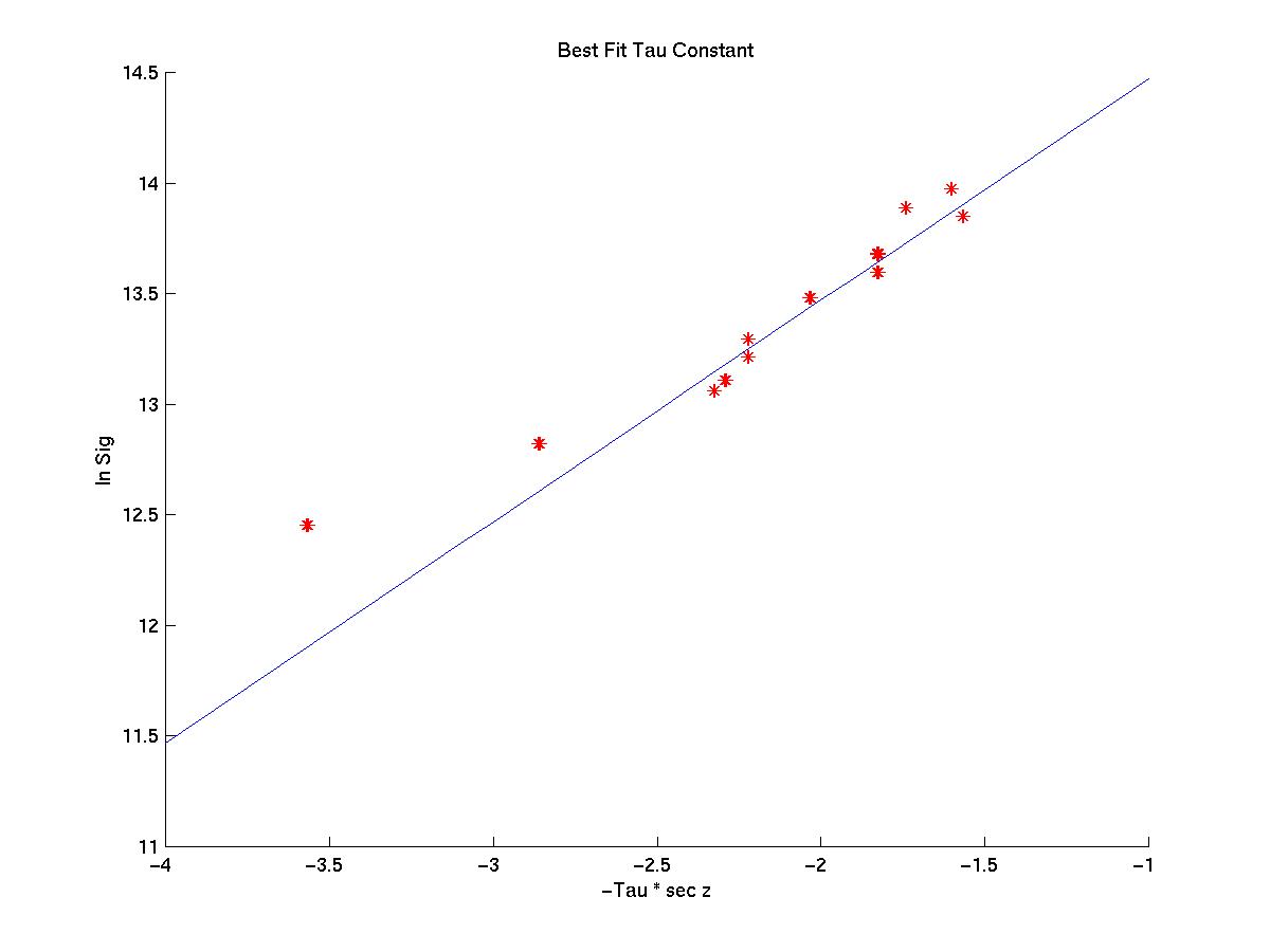
The same methodology was used to obtain constants using 13 different observations of Ngc 6334. The slope, or X, of that line, after adjusting the errors, was .89 (+/- .1). The reduced Chi squared was initially 2.1, so again I adjusted it to 1 and bumped the standard deviations up to average. Before adjusting the errors the slope was .98, so I was hesitant to trust the .89 measurement of X. I used the slope of 1 from the Sgr B2 data, and I estimated a y-intercept of 15.47 (+/- .21). The graph is following.
From the y-intercept (ln So Y) of the previous graph, we can extract a value of Y, using our estimate of So for Ngc 6334 from Gezari's paper. This gives us a Y of 421.02 (+/- 101.09) integ-units/Jy. This constant will enable us to convert from integ-units to an actual physical measurement in Janskys for a given observation. Working backwards, then, with Sgr B2, we can estimate a source flux of 51396 Jy (+/- 15423.3 Jy) per 5' beam. One may recall that a 5' beam is merely an estimate. The following is a summary of the constants for different beam sizes and for different sources.
| Beam Size | Y (integ-units/Jy) |
| 4' | 524.82 (+/- 122.53) |
| 5' | 421.02 (+/- 101.09) |
| 6' | 312.14 (+/- 312.14) |
| Source | X |
| Ngc 6334 | 1 (+/- .08) |
| Sgr B2 | .89 (+/- .1) |
One good thing to ask is if these constants, especially Y, are changing with time. This would indicate that for certain reasons, quite possibly snow on the tertiary, the signal strength is varying. Since we know the signal measured for each observation, as well as the tau and the zenith angle, we can plot SoY. Taking an average of So Y for all the observations during a day, we can see if there is a trend with time. In the following graph of So Y for Sgr B2, the reference line is So Y extracted from the previous best-fit line.
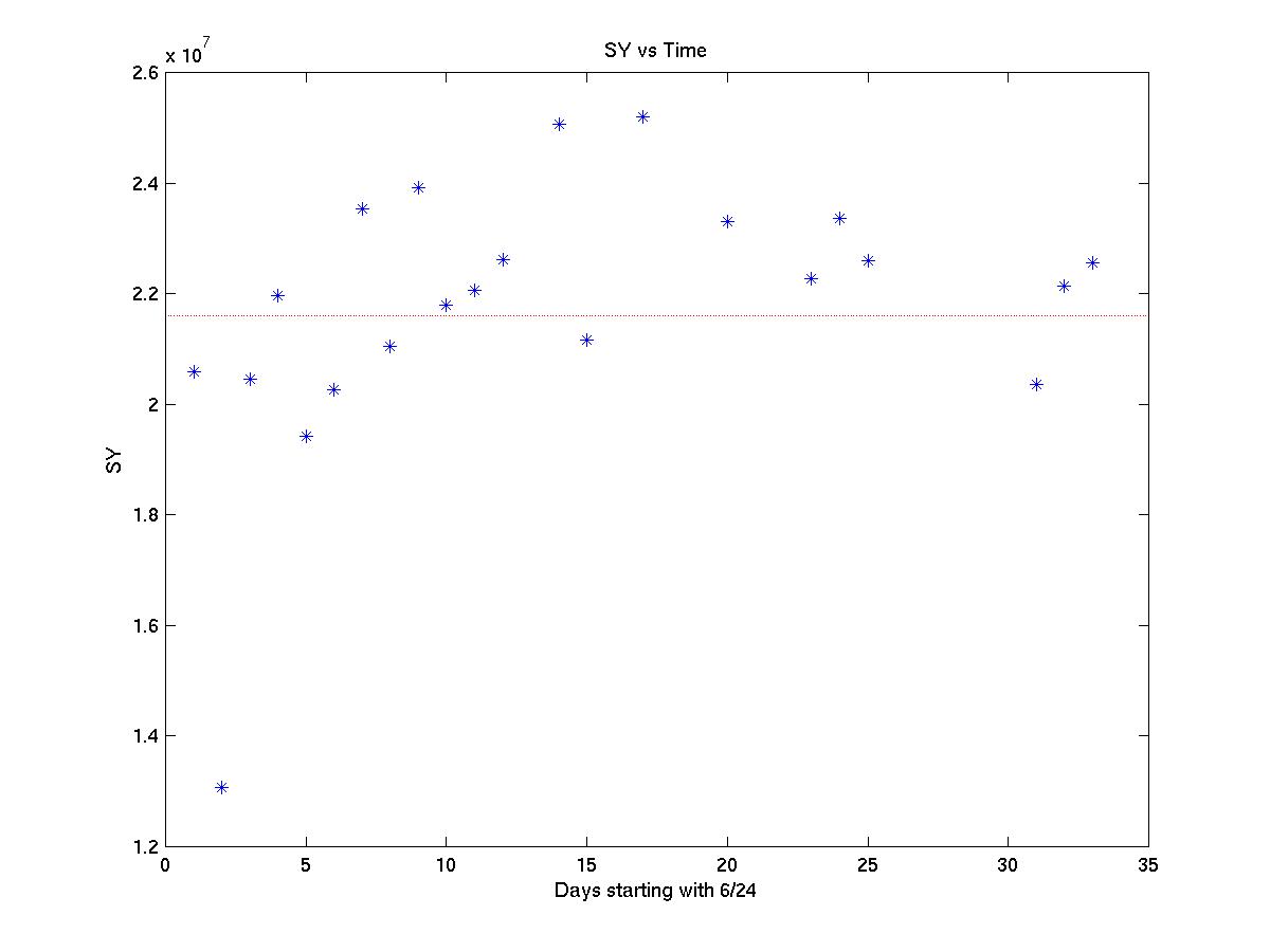
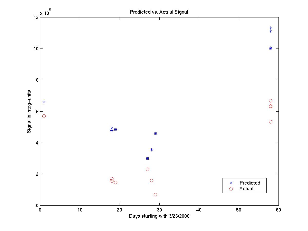
There might be a slight trend in the with time, but it does not seem to be significant. The biggest difference from the reference line is about .2 * 10^7, which is fairly small compared with the variations during a single day of measurements, which is approximately .5 * 10^7. This, then, is a good sign that the data taken during June and July for Sgr B2 is fairly consistent. The same thing can be seen if a graph is made of SoY for Ngc 6334. However, the first sets of data from April and May were inconsitent with tau. Plotting the predicted signal for a 5' beam and comparing it with the actual signal in integ-units received, we can conclude that the signal in April and May was inconsistently low. A small layer of snow on the tertiary can change the signal drastically, which could certainly account for the varying signals. Also, this data was taken at a time when the pointing and focus were still being determined. There are many plausible sources for systematic errors.
So, with the ability to calibrate photometry data, there are several things that can be determined. Looking at an arbitrary source, we can determine its flux, and thus the power that reaches the telescope. A parameter called the NEFD (Noise Equivalent Flux Density), an estimate of how long a certain souce must be observed to obtain a certain noise level, is determined using polarimetry data and a measurement of the source flux. We can also work backwards, converting the signal in integ-units to Watts, a measurement of the power received in the SPARO detectors. Since we can determine the flux and thus the power incident to the telescope, we can take the ratio of the power incident and received, determining the Viper telescope transmission. For each of the 104 different measurements of Sgr B2 and the 14 different measurements of Ngc 6334, I calculated a ratio of the power incident and received. I then found the average calculated transmission for these two sources. A more detailed description can be found here.
| Source | Calculated Tranmission |
| Ngc 6334 | 49.08 |
| Sgr B2 | 46.06 |
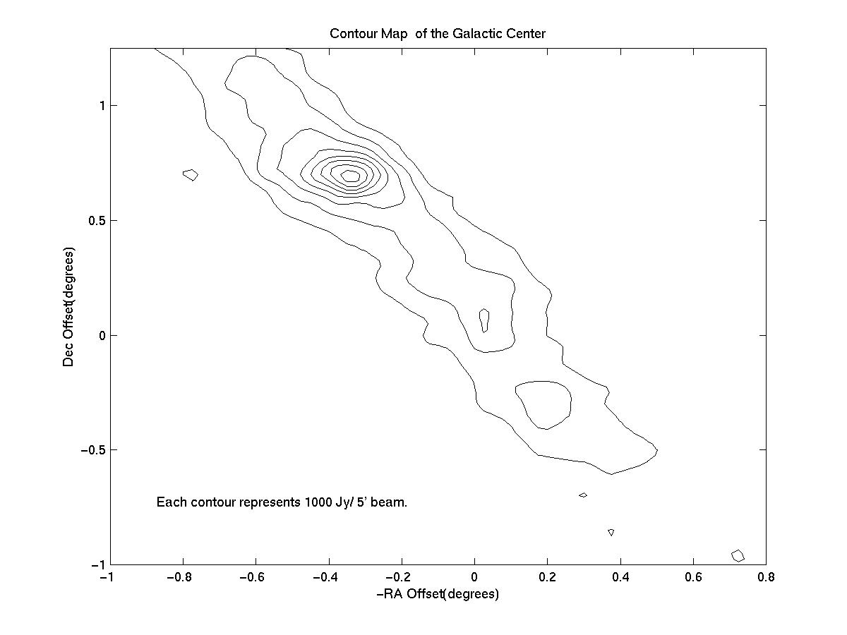
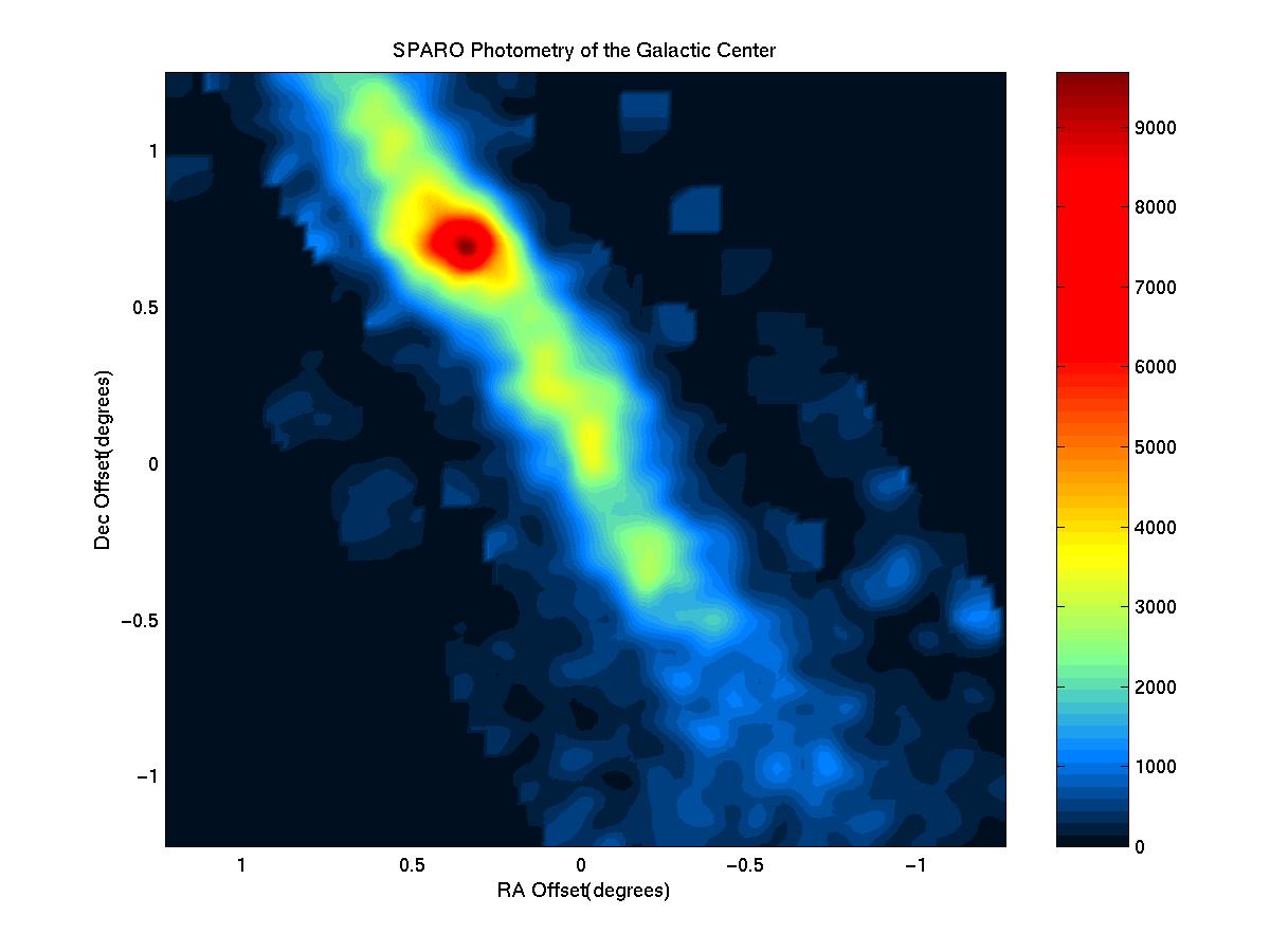
While the ultimate goal of SPARO is to map the magnetic field of the galactic center on a large scale, a smaller goal was the calibration of its photometric observations. With the ability to calibrate photometry data, many more things can be determined, such as the NEFD and the telescope transmission. In addition, consistent photometry data indicates to a certain degree consistent polarimetry data. More information concerning the calibration of polarimetry data is available here. Plus, there remains an even simpler reason to calibrate photometry data--to make photometry maps. The following is a contour map of the galactic center from an observation on May 20,2000. A color map is available here.